Distributions

Statistics work with the concept or random variable. We can imagine a random variable like a process which generates numbers but we do not know precisely the generated value. This analogy works fine, even when we think at observing something. Let work that by an example.

Imagine that we measure the heights of some men from a given place. We notice and collect some values. We might ask which is the process that generated the heights? Since we measured something, but the values are out of our control, the question is legitimate. The answer is the total number of factors which influenced the height of a men, including genes, culture, climate, longitude and latitude, and so on. All those imaginable factors together can be seen as a process which determines the heights.

Now we identified which is the process. The next legitimate question is why random? Since there are a lot of factors inside the process, we usually are in the situation where we don't understand the underlying mechanics of the process. This can happen because we did not identified all the determinant factors. This can also happen simply because it is too complex. And there are also cases when we simply do not want or can't understand. Because of that we simply can't determine precisely the height of an individual men starting from known factors.

We can't do that for individual, but we can say something more when more individuals are analyzed. Statistics is about populations (the total set of observations) and samples (a part of the existent samples), not about individuals. Thus when we talk about an individual we talk through the lenses of population. And because it's not precise we name it random.

A random variable can be described in many ways, but all those formulations maps a potential interval of observable values with a probability. What we know when we have a random variable is a set of potential observable values and probability assigned with those values.

Normal distribution

Normal or Gaussian distribution is perhaps the most known distribution. It is the distribution of the bell shape, even thought it is not unique among bell shaped distributions.

The implementation of normal distribution lies in:rapaio.core.distributions.Normal.

// build a normal distribution with mean = 2, and standard deviation = 3
Normal normal = new Normal(2,3);

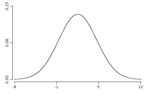
Normal distribution defined by two independent parameters: mean and standard deviation. Mean tells us when is the center of the distribution and standard deviation is a measure of variability.

We can generate a random sample from this distribution.

RandomSource.setSeed(1);
Numeric x = normal.sample(100).withName("x");
x.printSummary();

> printSummary(var: x)
name: x
type: NUMERIC
rows: 100, complete: 100, missing: 0
   Min. : -5.722
1st Qu. : -0.441
 Median :  2.040
   Mean :  1.927
2nd Qu. :  3.680
   Max. : 11.254

We can notice that the sample mean is 1.927, which is close to the population mean, but not equal. This is as expected. Since we generated a set of random values we can't expect to have a sample mean identical with population mean. If we expect that than we can suspect the generated numbers are not random.

WS.draw(funLine(normal::pdf).xLim(-8, 12).yLim(0, 0.15));

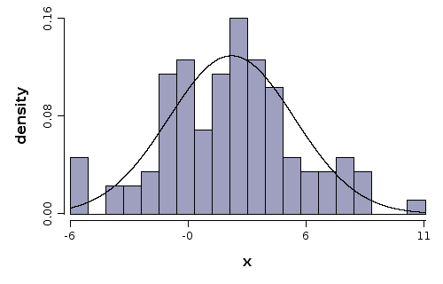
We draw now a histogram built from the generated sample, and the distribution which was used to generate values:

WS.draw(hist(x, prob(true), bins(20)).funLine(normal::pdf));

Student t distribution

Student t distribution is one of the most important distributions related with normal distribution. You can interpret the t distribution as a normal distribution, with additional uncertainty in the variance parameter.

Suppose that we are interested in the mean of a random sample normally distributed. If we know the mean and standard deviation of the population, than we could emply a z test. But often is the case where we do not know the standard deviation. What we can do? We can use a plug in estimated value for the standard deviation. The problem is that the estimated value of the standard deviation is not given anymore, it is not a given parameter of the population. Instead, it is an estimated value of that parameter, which implies the fact that it contains some error. This is the t distribution.

Formally the t distribution can be described as:

$T = \frac{Z}{\sqrt{V / \nu}}$

where $Z \sim N(0,1)$, $V \sim {\chi}^2_\nu$ and $Z$ and $V$ are independent.

What is important to note here is that the degrees of freedom $\nu$ does not depend on $\mu$ or $\sigma$, parameters of the original population. This is what makes this distribution important in practice.

To increase the understanding of this intuition we will draw a normal distribution and several t distributions with various degrees of freedom.

Normal n = new Normal();
StudentT t1 = new StudentT(1);
StudentT t2 = new StudentT(2);
StudentT t10 = new StudentT(10);
StudentT t100 = new StudentT(100);

Plot p = funLine(n::pdf, color(1))
        .funLine(t1::pdf, color(2))
        .funLine(t2::pdf, color(3))
        .funLine(t10::pdf, color(4))
        .funLine(t100::pdf, color(5))
        .xLim(-10, 10).yLim(0, 0.45)
        .legend(3, 0.4, color(1, 2, 3, 4, 5), labels("normal", "t1", "t2", "t10", "t100"));

WS.draw(p);

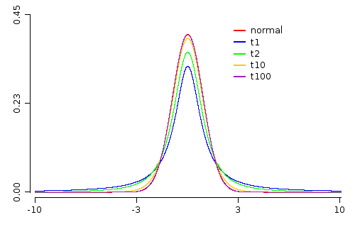
Looking at the image above we see that the standard normal distribution has the highest value at $0$. We note also that the t distribution with 1 degree of freedom has the lowest value at $0$. As the degrees of freedom increases the value at $0$ increases as well.

The reverse is true when we are looking for tails. The t with 1 degree of freedom has the fattest tail. This means that it have the highest uncertainty.

To illustrate better the concept, we compute the 0.975 quantiles of those distributions:

Normal n = new Normal();
StudentT t1 = new StudentT(1);
StudentT t2 = new StudentT(2);
StudentT t10 = new StudentT(10);
StudentT t100 = new StudentT(100);

Var dist = Nominal.copy(
        n.name(), t100.name(), t10.name(), 
        t2.name(), t1.name())
        .withName("distr");
Var p1 = Numeric.copy(
        n.quantile(0.975), t100.quantile(0.975), t10.quantile(0.975), 
        t2.quantile(0.975), t1.quantile(0.975))
        .withName("q0.975");
SolidFrame.byVars(dist, p1).printLines();

                  distr                    q0.975      
 [0]              Normal(mu=0, sd=1)   1.95996398454005
 [1] StudentT(df=100, mu=0, sigma=1)   1.98397151852356
 [2]  StudentT(df=10, mu=0, sigma=1)   2.22813885198627
 [3]   StudentT(df=2, mu=0, sigma=1)   4.30265272974946
 [4]   StudentT(df=1, mu=0, sigma=1)  12.70620473617469

We can see that if the degrees of freedom increases the quantiles decreases and is getting closer to the values of normal distribution. Often the degrees of freedom is computed from the sample size in one way or another. That means the t distribution is getting closer to a normal distribution if the sample is large. Often when we are dealing with samples of size over $100$ the t distribution gives almost the same results ad the normal distribution. As a consequence normal distribution can be used as an approximation if the sample size is large.