Tree model

Building models in the manual way is often not the way to go. This process is tedious and time consuming. There are already built automated procedures, which incorporate miscellaneous approaches to learn a classifier. One of the often used models is the decision tree. Decision trees are greedy local approximations build in a recursive greedy fashion. Often the split decision at node level uses a single feature. At leave nodes a simple majority classifier creates the classification rule.

Gender model with decision tree

Initially we will build a CART decision tree using as input feature the Sex variable. We do this to exemplify how a manual rule can be created in an automated fashion.

Frame tr = train.mapVars("Survived,Sex");
CTree tree = CTree.newCART();
tree.train(tr, "Survived");
tree.printSummary();

CTree model
================

Description:
CTree {varSelector=VarSelector[ALL];
minCount=1;
maxDepth=-1;
tests=ORDINAL:NumericBinary,INDEX:NumericBinary,BINARY:BinaryBinary,NOMINAL:Nominal_Binary,NUMERIC:NumericBinary;
func=GiniGain;
split=ToAllWeighted;
}

Capabilities:
types inputs/targets: BINARY,INDEX,NOMINAL,NUMERIC/NOMINAL
counts inputs/targets: [1,1000000] / [1,1]
missing inputs/targets: true/false

Learned model:
input vars: 

 0. Sex : NOMINAL  |

target vars:
> Survived : NOMINAL [?,0,1]

total number of nodes: 3
total number of leaves: 2
description:
split, n/err, classes (densities) [* if is leaf / purity if not]

|- 1. root    891/342 0 (0.616 0.384 ) [0.139648]
|   |- 2. Sex == female    314/81 1 (0.258 0.742 ) *
|   |- 3. Sex != female    577/109 0 (0.811 0.189 ) *

Taking a closer look at the last three rows from the output, one can identify our manual rule. Basically the interpretation is: "all the females survived, all the males did not". For exemplification purposes we build also the submit file.

// fit the tree to test data frame
CFit fit = tree.fit(test);
// build teh submission 
Frame submit = SolidFrame.wrapOf(
        // use original ids
        test.var("PassengerId"), 
        // use class prediction from fit
        fit.firstClasses().solidCopy().withName("Survived")  
);
// write to a submit file
new Csv().withQuotes(false).write(submit, root + "tree1-model.csv");

Enrich tree by using other features

Our training data set has more than a single input feature. Thus We can state we didn't use all the information available. We will add now the class and embarking port and see how it behaves.

Frame tr = train.mapVars("Survived,Sex,Pclass,Embarked");

CTree tree = CTree.newCART();
tree.train(tr, "Survived");
tree.printSummary();

CFit fit = tree.fit(test);
Frame submit = SolidFrame.wrapOf(
        test.var("PassengerId"),
        fit.firstClasses().withName("Survived")
);
new Csv().withQuotes(false).write(submit, root + "tree2-model.csv");

This is the resulted tree:

Capabilities:
types inputs/targets: BINARY,INDEX,NOMINAL,NUMERIC/NOMINAL
counts inputs/targets: [1,1000000] / [1,1]
missing inputs/targets: true/false

Learned model:
input vars: 

 0. Sex : NOMINAL  | 1. Pclass : NOMINAL  | 2. Embarked : NOMINAL  |

target vars:
> Survived : NOMINAL [?,0,1]

total number of nodes: 35
total number of leaves: 18
description:
split, n/err, classes (densities) [* if is leaf / purity if not]

|- 1. root    891/342 0 (0.616 0.384 ) [0.139648]
|   |- 2. Sex == female    314/81 1 (0.258 0.742 ) [0.0204665]
|   |   |- 3. Pclass == 2    76/6 1 (0.079 0.921 ) [0.0003369]
|   |   |   |- 4. Embarked == Q    2/0 1 (0 1 ) *
|   |   |   |- 5. Embarked != Q    74/6 1 (0.081 0.919 ) [0.0013737]
|   |   |   |   |- 6. Embarked == C    7/0 1 (0 1 ) *
|   |   |   |   |- 7. Embarked != C    67/6 1 (0.09 0.91 ) *
|   |   |- 8. Pclass != 2    238/75 1 (0.315 0.685 ) [0.1047167]
|   |   |   |- 9. Pclass == 1    94/3 1 (0.032 0.968 ) [0.0000234]
|   |   |   |   |- 10. Embarked == Q    1/0 1 (0 1 ) *
|   |   |   |   |- 11. Embarked != Q    93/3 1 (0.032 0.968 ) [0.000169]
|   |   |   |   |   |- 12. Embarked == C    43/1 1 (0.023 0.977 ) *
|   |   |   |   |   |- 13. Embarked != C    50/2 1 (0.04 0.96 ) *
|   |   |   |- 14. Pclass != 1    144/72 1 (0.5 0.5 ) [0.0307125]
|   |   |   |   |- 15. Embarked == Q    33/9 1 (0.273 0.727 ) *
|   |   |   |   |- 16. Embarked != Q    111/48 0 (0.568 0.432 ) [0.0252406]
|   |   |   |   |   |- 17. Embarked == C    23/8 1 (0.348 0.652 ) *
|   |   |   |   |   |- 18. Embarked != C    88/33 0 (0.625 0.375 ) *
|   |- 19. Sex != female    577/109 0 (0.811 0.189 ) [0.0020493]
|   |   |- 20. Embarked == Q    41/3 0 (0.927 0.073 ) [0.0002677]
|   |   |   |- 21. Pclass == 2    1/0 0 (1 0 ) *
|   |   |   |- 22. Pclass != 2    40/3 0 (0.925 0.075 ) [0.0002885]
|   |   |   |   |- 23. Pclass == 1    1/0 0 (1 0 ) *
|   |   |   |   |- 24. Pclass != 1    39/3 0 (0.923 0.077 ) *
|   |   |- 25. Embarked != Q    536/106 0 (0.802 0.198 ) [0.0049791]
|   |   |   |- 26. Embarked == C    95/29 0 (0.695 0.305 ) [0.0026071]
|   |   |   |   |- 27. Pclass == 2    10/2 0 (0.8 0.2 ) *
|   |   |   |   |- 28. Pclass != 2    85/27 0 (0.682 0.318 ) [0.014825]
|   |   |   |   |   |- 29. Pclass == 1    42/17 0 (0.595 0.405 ) *
|   |   |   |   |   |- 30. Pclass != 1    43/10 0 (0.767 0.233 ) *
|   |   |   |- 31. Embarked != C    441/77 0 (0.825 0.175 ) [0.0002248]
|   |   |   |   |- 32. Pclass == 2    97/15 0 (0.845 0.155 ) *
|   |   |   |   |- 33. Pclass != 2    344/62 0 (0.82 0.18 ) [0.0180924]
|   |   |   |   |   |- 34. Pclass == 1    79/28 0 (0.646 0.354 ) *
|   |   |   |   |   |- 35. Pclass != 1    265/34 0 (0.872 0.128 ) *

The tree is much richer and there are more chances to be better. This is what happened after submission.

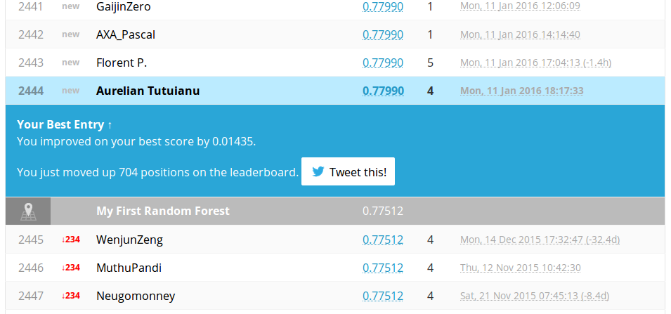
Nice!. We advanced $704$ positions and improved our score with $0.01435$. On public leader board we have a nice $0.77990$ accuracy score.

Overfitting with trees

What about using other input features to improve our prediction accuracy? There are some of them which we can include directly, with no changes: Age,Fare,SibSp and Parch.

We can change the script slightly, to include those new input features. But we can do better, we can use cross-validation to estimate what will happen.

CTree tree = CTree.newCART();
CEvaluation.cv(train.mapVars("Survived,Sex,Pclass,Embarked"),
        "Survived", tree, 10);
CEvaluation.cv(train.mapVars("Survived,Sex,Pclass,Embarked,Age,Fare,SibSp,Parch"),
        "Survived", tree, 10);

CrossValidation with 10 folds
...
Mean accuracy:0.811473
SE: 0.034062     (Standard error)

CrossValidation with 10 folds
...
Mean accuracy:0.774370
SE: 0.046494     (Standard error)

Notice that the 10-crossfold estimator of the accuracy has dropped with a large quantity. What happens? We can have an idea if we take a look at the learned tree:

tree.train(train.mapVars("Survived,Sex,Pclass,Embarked,Age,Fare,SibSp,Parch"), "Survived");
tree.printSummary();

total number of nodes: 1197
total number of leaves: 599
description:
split, n/err, classes (densities) [* if is leaf / purity if not]

|- 1. root    891/342 0 (0.616 0.384 ) [0.139648]
|   |- 2. Sex == female    314/81 1 (0.258 0.742 ) [0.0282131]
|   |   |- 3. Fare <= 48.2    225/76 1 (0.338 0.662 ) [0.0645841]
|   |   |   |- 4. Pclass == 2    74/6 1 (0.081 0.919 ) [0.0099206]
|   |   |   |   |- 5. Age <= 56    73/5 1 (0.069 0.931 ) [0.0036241]
|   |   |   |   |   |- 6. Age <= 23.5    22/0 1 (0 1 ) *
|   |   |   |   |   |- 7. Age > 23.5    53/5 1 (0.095 0.905 ) [0.0066092]
|   |   |   |   |   |   |- 8. Age <= 27.5    14/3 1 (0.243 0.757 ) [0.0138889]
|   |   |   |   |   |   |   |- 9. Age <= 25.5    10/1 1 (0.122 0.878 ) [0.0004053]
|   |   |   |   |   |   |   |   |- 10. Fare <= 13.75    3/1 1 (0.474 0.526 ) [0.0249307]
|   |   |   |   |   |   |   |   |   |- 11. Embarked == Q    1/0 1 (0 1 ) *
|   |   |   |   |   |   |   |   |   |- 12. Embarked != Q    2/1 1 (0.5 0.5 ) *
|   |   |   |   |   |   |   |   |- 13. Fare > 13.75    7/0 1 (0 1 ) *
|   |   |   |   |   |   |   |- 14. Age > 25.5    6/2 1 (0.486 0.514 ) [0.1635168]
|   |   |   |   |   |   |   |   |- 15. Fare <= 17.42915    3/0 1 (0 1 ) *
|   |   |   |   |   |   |   |   |- 16. Fare > 17.42915    3/1 0 (0.973 0.027 ) [0.001384]
|   |   |   |   |   |   |   |   |   |- 17. Fare <= 29.5    2/0 0 (1 0 ) *
|   |   |   |   |   |   |   |   |   |- 18. Fare > 29.5    1/0 1 (0 1 ) *
|   |   |   |   |   |   |- 19. Age > 27.5    41/2 1 (0.05 0.95 ) [0.0061363]
|   |   |   |   |   |   |   |- 20. Age <= 37    26/0 1 (0 1 ) *

...

|   |   |   |   |   |   |   |   |   |   |- 1189. Fare > 28.275    3/0 1 (0 1 ) *
|   |   |   |   |   |   |   |   |- 1190. Fare > 30.5979    13/3 0 (0.769 0.231 ) [0.1140039]
|   |   |   |   |   |   |   |   |   |- 1191. Pclass == 1    10/1 0 (0.9 0.1 ) [0.0085714]
|   |   |   |   |   |   |   |   |   |   |- 1192. Fare <= 37.55    4/1 0 (0.75 0.25 ) [0.125]
|   |   |   |   |   |   |   |   |   |   |   |- 1193. Fare <= 35.25    3/0 0 (1 0 ) *
|   |   |   |   |   |   |   |   |   |   |   |- 1194. Fare > 35.25    1/0 1 (0 1 ) *
|   |   |   |   |   |   |   |   |   |   |- 1195. Fare > 37.55    6/0 0 (1 0 ) *
|   |   |   |   |   |   |   |   |   |- 1196. Pclass != 1    3/1 1 (0.333 0.667 ) *
|   |   |   |   |- 1197. SibSp > 2.5    15/0 0 (1 0 ) *

Notice how large is the tree. Basically the tree was full grown and overfit the training data set too much. We can ask ourselves why that happens? Why it happens now, and did not happened when we had fewer inputs? The answer is that it happened also before. But it's consequences were not so drastic.

The first tree used for training just $3$ input nominal features. Notice that all three features are nominal. The maximum number of groups which one can form is given by the product of the number of levels for each feature. This total maximal number is $2*3*3=18$. It practically exhausted the discrimination potential of those features. It did overfit in that reduced space of features. When we apply the model to the whole data set, the effect of exhaustion is not seen anymore.

The second tree does the same thing, but this time in a richer space, with added input dimensions. Compared with the full feature space, we see the effect.

There are two approaches to avoid overfit for a decision tree. The first approach is to stop learning up to the moment when we exhaust the data. The name for this approach is early stop. We can do that by specifying some parameters of the tree model:

• Set a minimum number of instances for leaf node
• Set a maximal depth for the tree
• Not implemented yet, but easy to do: complexity threshold, maximal number of nodes in a tree

The second approach is to prune the tree. Pruning procedure consists of growing the full tree and later on removing some nodes if they do not provide some type of gain. Currently we implemented only reduced error pruning strategy.

We will test with 10-fold cross validation an early-stopping strategy to see how it works.

CEvaluation.cv(train.mapVars("Survived,Sex,Pclass,Embarked,Age,Fare,SibSp,Parch"),
        "Survived", tree.withMaxDepth(12).withMinCount(4), 10);

Mean accuracy:0.796854
SE: 0.034929     (Standard error)

I tried some values, just to show that we can do something about it, but the progress did not appear. We should try a different approach, and that is an ensemble. Next session contains directions on how to build such an ensemble.