Stacking classifiers

Using random forests or SVMs did not provided us with a result over $0.8$. We have two very different types of models which performed well. For the sole purpose of prediction we use a nice ensemble technique which often provides good prediction performance gain. This technique is called stacking.

The idea behind stacking is that one can explore the space of the solutions with different approaches. Each approach (or statistical model) is basically an interpretation of the solution. But often times a proper interpretation is really hard to find. Each interpretation of the solution can have good points and weak points. The idea is to blend those interpretations into a single one in a way that we try somehow to keep what is string from each individual classifier.

A stacking classifier take some base learners and train them on training data. The results of the base learners are used as input for a stacking learner. This stacking learner is trained on the output of base learners and target variable and is finally used for prediction.

Classifier model = new CStacking()
        .withLearners(
                new BinarySMO()
                        .withInputFilters(inputFilters)
                        .withC(1)
                        .withTol(1e-10)
                        .withKernel(new CauchyKernel(20)),
                CForest.newRF()
                        .withInputFilters(inputFilters)
                        .withMCols(4)
                        .withBootstrap(0.07)
                        .withClassifier(CTree.newCART()
                            .withFunction(CTreePurityFunction.GainRatio)
                            .withMinGain(0.001))
                        .withRuns(200)
        ).withStacker(CForest.newRF().withBootstrap(0.3)
            .withRuns(200)
            .withClassifier(CTree.newCART()
                .withFunction(CTreePurityFunction.GainRatio)
                .withMinGain(0.05)));

Usually one uses a binary logistic regression model but it provided weak results. What looked much better is another random forrest classifier. However the stacking model uses a big value for minimum gain parameter because we want to act as an draft average over the results.

> Confusion

 Ac\Pr |    0    1 | total
 ----- |    -    - | -----
     0 | >522   27 |   549
     1 |   87 >255 |   342
 ----- |    -    - | -----
 total |  609  282 |   891


Complete cases 891 from 891
Acc: 0.8720539         (Accuracy )
F1:  0.9015544         (F1 score / F-measure)
MCC: 0.7281918         (Matthew correlation coefficient)
Pre: 0.8571429         (Precision)
Rec: 0.9508197         (Recall)
G:   0.902767         (G-measure)
Cross validation 10-fold
CV fold: 1, acc: 0.888889, mean: 0.888889, se: NaN
CV fold: 2, acc: 0.786517, mean: 0.837703, se: 0.072388
CV fold: 3, acc: 0.842697, mean: 0.839367, se: 0.051267
CV fold: 4, acc: 0.820225, mean: 0.834582, se: 0.042940
CV fold: 5, acc: 0.808989, mean: 0.829463, se: 0.038908
CV fold: 6, acc: 0.853933, mean: 0.833541, se: 0.036206
CV fold: 7, acc: 0.786517, mean: 0.826824, se: 0.037527
CV fold: 8, acc: 0.898876, mean: 0.835830, se: 0.043082
CV fold: 9, acc: 0.831461, mean: 0.835345, se: 0.040326
CV fold:10, acc: 0.775281, mean: 0.829338, se: 0.042500
=================
mean: 0.829338, se: 0.042500

Again, the results are promising. The space between training error and cross validation error is smaller and our expectations grows.

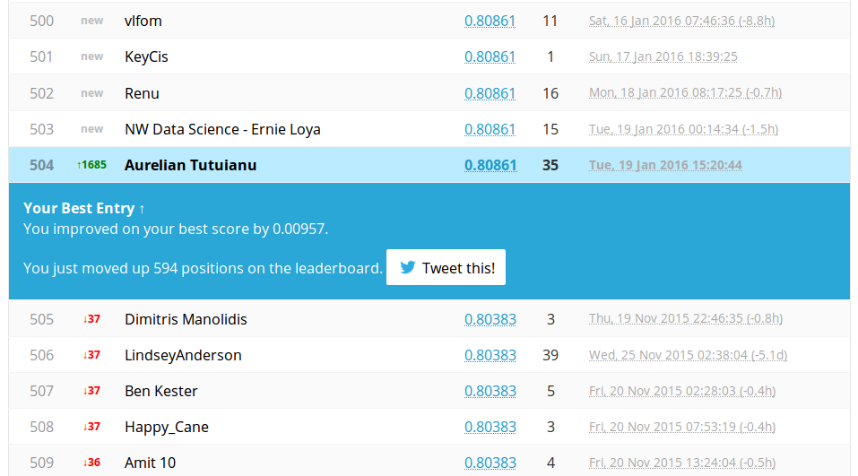
Finally our target performance was achieved!!

Note:

The general advice in real life is to not fight for each piece of performance measure. It really depends on the question one wants to answer. Often measures like ROC or partial ROC are much better than error frequency. We fixed this milestone because we know it is possible and because it looks like a psychological difficulty. (that $0.799$ is outrageous).